Data Home | Math Topics | Environment Topics | Topics Matrix | Master List | Help | Feedback

Download the Data

RichText File

Excel File

Text File

Minitab File

Data Set #049

About the Data
View the Data
Help with Using Data
Play with the data on StatCrunch
 

  Go to Top  

About the Data

    An important class of distributions or density curves in statistics is the normal distribution.  All normal distributions have the same overall shape that is often referred to as "bell shaped".  These shapes are symmetric about the center, which is the location of the mean, median and mode of the data set.   
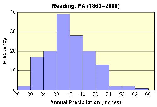
It appears that the precipitation frequency distribution for Reading is  "almost normal" since it is almost symmetric about the center and has a bell-shaped appearance.  If students were to display precipitation distributions for other cities, many of these would also have the same bell-shaped curve.   Why is this so?  The answer lies in the fact that precipitation amounts, like many other natural phenomena, are the result of many random factors. When this is the case, we expect a normal distribution.

    Mentioned above was the fact that the center of a normal distribution is the mean.  The mean annual precipitation for the years 1863 to 1999 was 41.5 inches, which looks about right on the Excel histogram.   It's quite obvious that the center (mean) for the Reading distribution would be quite different than the center for a much drier city such as Salt Lake or Phoenix.  Also,  a city whose precipitation from year to year is more consistent or more varied would have a histogram that is narrower or wider, respectfully.  So even though normal distributions have the same overall shape, they may have different centers (means) and have different widths (deviations from the mean).  The width of a normal distribution is quantified by computing the standard deviation. For the Reading data, the standard deviation is 6.5 inches.  (The formula to compute this number is not given here, but can be found in any basic statistics text.  Also, most calculators, spreadsheets and statistics packages will compute the standard deviation.)

    If we denote the mean by m and the standard deviation by s, then any normal distribution can be described by the 68-95-99.7 rule.  This rule states that:  68% of the data will lie within 1s of the mean m, 95% of the data will lie within 2s of the mean m, and 99.7% of the data will lie within 3s of the mean m . We can use the 68-95-99.7 rule as a means to check "how normal" the precipitation data is for Reading.  This is a good student exercise.  We can also use properties of the normal distribution to answer a question such as, "How likely is it that the precipitation for Reading will be between 30 and 31 inches in any given year?".  Details are left for statistics courses.

    We obtained precipitation data for the lower 48 states from the United States Historical Climate Network (USHCN), part of NOAA's National Climate Data Center. The USHCN has historical records for 1221 weather station in the lower 48 states, of which 1182 are currently operational.  At the USHCN website one can download historical data sets that have varying amounts of editing. We downloaded the (gigantic) national precipitation data, selected the Filnet edited data, then divided the national data set into state-by-state sets.    Note:  The Filnet edited precipitation data  (1) has removed outliers more that 3 standard deviations from the period mean (2) has been adjusted to remove time of observation bias, the Maximum/Minimum Temperature System (MMTS) bias, station moves/changes bias and (3) contains estimated values for missing/outlier data.
Additionally, the USHCN provides weather station information (referred to as the Station Inventory information), with details about station location, history, measuring devices, personnel, reliability, etc.   We edited this file on a state by state basis to include only latitude, longitude, and elevation data for the latest location of each station.   To download state-by-state files, go to DataSet#050.  Those wishing to obtain a single national or unedited file should go to the USHCN website.

Data source: United States Historical Climate Network (USHCN)
http://www.ncdc.noaa.gov/ol/climate/research/ushcn/ushcn.html


  Go to Top  

View the Data


Reading, Pennsylvania Annual Precipitation


Source: US Historic Climate Network


year

precipitation (in.)


Bin

Frequency

1863

46.31


26

1

1864

38.42


30

1

1865

49.65


34

18

1866

41.51


38

19

1867

49.94


42

38

1868

48.43


46

29

1869

45.41


50

20

1870

48.62


54

8

1871

48.84


58

1

1872

43.90


62

1

1873

51.53


66

1

1874

35.87


More

0

1875

40.02


1876

39.61


Mean

41.48

1877

47.38


Median

40.99

1878

36.93


Mode

39.26

1879

41.79


Standard Deviation

6.52

1880

31.25


1881

40.06


1882

39.45


1883

40.86


1884

48.28


1885

39.03


1886

40.03


1887

42.88


1888

51.78


1889

64.72


1890

45.92


1891

48.79


1892

36.01


1893

38.39


1894

51.09


1895

33.07


1896

33.12


1897

47.91


1898

45.57


1899

44.48


1900

35.11


1901

43.68


1902

52.66


1903

45.91


1904

41.67


1905

38.38


1906

43.52


1907

44.11


1908

35.67


1909

31.88


1910

34.61


1911

45.11


1912

46.83


1913

42.66


1914

31.19


1915

44.42


1916

41.52


1917

32.84


1918

33.90


1919

41.20


1920

37.91


1921

35.32


1922

33.76


1923

31.22


1924

40.99


1925

40.11


1926

40.30


1927

35.78


1928

39.96


1929

40.27


1930

25.75


1931

32.23


1932

44.23


1933

43.27


1934

44.49


1935

37.83


1936

42.04


1937

41.39


1938

43.57


1939

40.44


1940

39.26


1941

31.12


1942

52.65


1943

32.39


1944

40.92


1945

48.98


1946

36.81


1947

44.53


1948

47.04


1949

37.97


1950

41.82


1951

43.73


1952

54.31


1953

49.12


1954

34.94


1955

42.82


1956

44.32


1957

30.99


1958

43.91


1959

35.89


1960

39.26


1961

38.58


1962

40.08


1963

33.22


1964

33.32


1965

27.01


1966

34.17


1967

38.21


1968

34.08


1969

39.08


1970

36.84


1971

45.45


1972

53.12


1973

50.12


1974

38.56


1975

52.86


1976

42.64


1977

42.65


1978

43.46


1979

48.08


1980

31.84


1981

33.97


1982

40.18


1983

49.08


1984

47.85


1985

39.90


1986

45.43


1987

39.80


1988

38.32


1989

47.24


1990

46.00


1991

35.76


1992

39.08


1993

47.78


1994

49.18


1995

40.16


1996

60.46


1997

33.31


1998

41.89


1999

36.58


  Go to Top