About velocity versus discharge at Soos Creek
The size of a stream or river at any given point along the stream can be quantified by measuring
the width of the "wetted perimeter" of the channel, the mean depth of the water in the channel, and the
mean speed or velocity of the stream. These three measurements can be multiplied together to calculate the stream's
discharge at a station, which is the volume of water passing by in a given amount of time. Discharge is typically
measured in cubic meters or cubic feet per second, though in very low flows, gallons per minute might be used.
At a remote stream gauging station, the height of the water (gage height) is measured and
transmitted via satellite to a central recording facility. Empirical relationships (based on many measurements)
between gage height, velocity, mean depth and mean width are used to calculate discharge. Therefore, one key task
in this process is to actually measure mean velocity at various gage heights.
The velocity at any point in a river is controlled by a number of factors, including the
river's slope or gradient, roughness of the channel bed, turbulence of the flow, depth of the river, etc. Typically,
water moves faster away from the bed of the river, where obstacles create drag and turbulence. The highest velocity
overall is usually in the deepest part of the channel, just below the surface. And therefore the deeper the water,
the higher the velocity (for confined channel flow).
A river accommodates increasing discharge by widening, deepening and speeding up. Naturally
we would expect some sort of positive correlation between observed discharge and observed velocity. The data in
the table, collected by the United States Geological Survey for Soos Creek in Washington State, shows the expected
positive relationship. However, the relationship is highly non-linear. Velocity increases rapidly with increasing
discharge, but then flattens out, perhaps approaching some limit.
The best fit regression between discharge and velocity for Soos Creek approximates a simple
square root function, y = 0.25x 0.5 or y = 0.25*sqrt(x). However, the best fit regression does not match the "shape"
of the data that well. Using the graphing calculator, students can modify the two terms in this simple equation
to create power law functions with different shapes that might better represent the overall form of the data (though
with a lower correlation coefficient). Which parameter or parameters must be modified to give a "flatter"
curve? To give a more "hooked shaped" curve at low discharges? To shift the curve to the right?
What happens when the discharge is zero? What would cause an upper limit to velocity?
Reference: United States Geological Survey http://www.usgs.gov/